Coordinate system - these are two mutually perpendicular coordinate lines intersecting at the point that is the origin for each of them.

Coordinate axes are the lines that form the coordinate system.

abscissa(x-axis) is the horizontal axis.

Y-axis(y-axis) is the vertical axis.

Function

Function is a mapping of the elements of the set X to the set Y . In this case, each element x of the set X corresponds to one single value y of the set Y .

Straight

Linear function is a function of the form y = a x + b where a and b are any numbers.

The graph of a linear function is a straight line.

Consider how the graph will look depending on the coefficients a and b:

If a a > 0 , the line will pass through the I and III coordinate quarters.

If a a< 0 , прямая будет проходить через II и IV координатные четверти.

b is the point of intersection of the line with the y-axis.

If a a = 0 , the function becomes y = b .

Separately, we select the graph of the equation x \u003d a.

Important: this equation is not a function, since the definition of the function is violated (the function associates each element x of the set X with a single value y of the set Y). This equation associates one element x with an infinite set of elements y . However, the graph of this equation can be plotted. Let's just not call it the proud word "Function".

Parabola

The graph of the function y = a x 2 + b x + c is parabola .

In order to unambiguously determine how the parabola graph is located on the plane, you need to know what the coefficients a, b, c affect:

1. The coefficient a indicates where the branches of the parabola are directed.

• If a > 0 , the branches of the parabola are directed upwards.
• If a< 0 , ветки параболы направлены вниз.

1. The coefficient c indicates at what point the parabola intersects the y axis.
2. The coefficient b helps to find x in - the coordinate of the top of the parabola.

x in \u003d - b 2 a

1. The discriminant allows you to determine how many points of intersection a parabola has with an axis.

• If D > 0 - two points of intersection.
• If D = 0 - one point of intersection.
• If D< 0 — нет точек пересечения.

The graph of the function y = k x is hyperbola .

A characteristic feature of a hyperbola is that it has asymptotes.

Asymptotes of a hyperbola - straight lines, to which it tends, going to infinity.

The x-axis is the horizontal asymptote of the hyperbola

The y-axis is the vertical asymptote of the hyperbola.

On the graph, the asymptotes are marked with a green dotted line.

If the coefficient k > 0, then the branches of the hyperola pass through the I and III quarters.

If k<     0, ветви гиперболы проходят через II и IV четверти.

The smaller the absolute value of the coefficient k (the coefficient k without taking into account the sign), the closer the branches of the hyperbola to the x and y axes.

Square root

The function y     =     x has the following graph:

Increasing/decreasing functions

Function y   =   f(x) increases over the interval if a larger value of the argument (a larger x value) corresponds to a larger function value (a larger y value) .

That is, the more (to the right) x, the more (higher) y. Graph rises (look from left to right)

Function y   =   f(x) decreases over the interval if a larger argument value (a larger x value) corresponds to a smaller function value (a larger y value) .

Knowledge basic elementary functions, their properties and graphs no less important than knowing the multiplication table. They are like a foundation, everything is based on them, everything is built from them, and everything comes down to them.

In this article, we list all the main elementary functions, give their graphs and give them without derivation and proofs. properties of basic elementary functions according to the scheme:

• behavior of the function on the boundaries of the domain of definition, vertical asymptotes (if necessary, see the article classification of break points of a function);
• even and odd;
• convexity (convexity upwards) and concavity (convexity downwards) intervals, inflection points (if necessary, see the article function convexity, convexity direction, inflection points, convexity and inflection conditions);
• oblique and horizontal asymptotes;
• singular points of functions;
• special properties of some functions (for example, the smallest positive period for trigonometric functions).

If you are interested in or, then you can go to these sections of the theory.

Basic elementary functions are: constant function (constant), root of the nth degree, power function, exponential, logarithmic function, trigonometric and inverse trigonometric functions.

Page navigation.

Permanent function.

A constant function is given on the set of all real numbers by the formula , where C is some real number. The constant function assigns to each real value of the independent variable x the same value of the dependent variable y - the value С. A constant function is also called a constant.

The graph of a constant function is a straight line parallel to the x-axis and passing through a point with coordinates (0,C) . For example, let's show graphs of constant functions y=5 , y=-2 and , which in the figure below correspond to the black, red and blue lines, respectively.

Properties of a constant function.

• Domain of definition: the whole set of real numbers.
• The constant function is even.
• Range of values: set consisting of a single number C .
• A constant function is non-increasing and non-decreasing (that's why it is constant).
• It makes no sense to talk about the convexity and concavity of the constant.
• There is no asymptote.
• The function passes through the point (0,C) of the coordinate plane.

The root of the nth degree.

Consider the basic elementary function, which is given by the formula , where n is a natural number greater than one.

The root of the nth degree, n is an even number.

Let's start with the nth root function for even values ​​of the root exponent n .

For example, we give a picture with images of graphs of functions and , they correspond to black, red and blue lines.

The graphs of the functions of the root of an even degree have a similar appearance for other values ​​of the indicator.

Properties of the root of the nth degree for even n .

The root of the nth degree, n is an odd number.

The root function of the nth degree with an odd exponent of the root n is defined on the entire set of real numbers. For example, we present graphs of functions and , the black, red, and blue curves correspond to them.

For other odd values ​​of the root exponent, the graphs of the function will have a similar appearance.

Properties of the root of the nth degree for odd n .

Power function.

The power function is given by a formula of the form .

Consider the type of graphs of a power function and the properties of a power function depending on the value of the exponent.

Let's start with a power function with an integer exponent a . In this case, the form of graphs of power functions and the properties of functions depend on the even or odd exponent, as well as on its sign. Therefore, we first consider power functions for odd positive values ​​of the exponent a , then for even positive ones, then for odd negative exponents, and finally, for even negative a .

The properties of power functions with fractional and irrational exponents (as well as the type of graphs of such power functions) depend on the value of the exponent a. We will consider them, firstly, when a is from zero to one, secondly, when a is greater than one, thirdly, when a is from minus one to zero, and fourthly, when a is less than minus one.

In conclusion of this subsection, for the sake of completeness, we describe a power function with zero exponent.

Power function with odd positive exponent.

Consider a power function with an odd positive exponent, that is, with a=1,3,5,… .

The figure below shows graphs of power functions - black line, - blue line, - red line, - green line. For a=1 we have linear function y=x .

Properties of a power function with an odd positive exponent.

Power function with even positive exponent.

Consider a power function with an even positive exponent, that is, for a=2,4,6,… .

As an example, let's take graphs of power functions - black line, - blue line, - red line. For a=2 we have a quadratic function whose graph is quadratic parabola.

Properties of a power function with an even positive exponent.

Power function with an odd negative exponent.

Look at the graphs of the exponential function for odd negative values ​​​​of the exponent, that is, for a \u003d -1, -3, -5, ....

The figure shows graphs of exponential functions as examples - black line, - blue line, - red line, - green line. For a=-1 we have inverse proportionality, whose graph is hyperbola.

Properties of a power function with an odd negative exponent.

Power function with an even negative exponent.

Let's move on to the power function at a=-2,-4,-6,….

The figure shows graphs of power functions - black line, - blue line, - red line.

Properties of a power function with an even negative exponent.

A power function with a rational or irrational exponent whose value is greater than zero and less than one.

Note! If a is a positive fraction with an odd denominator, then some authors consider the interval to be the domain of the power function. At the same time, it is stipulated that the exponent a is an irreducible fraction. Now the authors of many textbooks on algebra and the beginnings of analysis DO NOT DEFINE power functions with an exponent in the form of a fraction with an odd denominator for negative values ​​of the argument. We will adhere to just such a view, that is, we will consider the domains of power functions with fractional positive exponents to be the set . We encourage students to get your teacher's perspective on this subtle point to avoid disagreement.

Consider a power function with rational or irrational exponent a , and .

We present graphs of power functions for a=11/12 (black line), a=5/7 (red line), (blue line), a=2/5 (green line).

A power function with a non-integer rational or irrational exponent greater than one.

Consider a power function with a non-integer rational or irrational exponent a , and .

Let us present the graphs of the power functions given by the formulas (black, red, blue and green lines respectively).

For other values ​​of the exponent a , the graphs of the function will have a similar look.

Power function properties for .

A power function with a real exponent that is greater than minus one and less than zero.

Note! If a is a negative fraction with an odd denominator, then some authors consider the interval . At the same time, it is stipulated that the exponent a is an irreducible fraction. Now the authors of many textbooks on algebra and the beginnings of analysis DO NOT DEFINE power functions with an exponent in the form of a fraction with an odd denominator for negative values ​​of the argument. We will adhere to just such a view, that is, we will consider the domains of power functions with fractional fractional negative exponents to be the set, respectively. We encourage students to get your teacher's perspective on this subtle point to avoid disagreement.

We pass to the power function , where .

In order to have a good idea of ​​the type of graphs of power functions for , we give examples of graphs of functions (black, red, blue, and green curves, respectively).

Properties of a power function with exponent a , .

A power function with a non-integer real exponent that is less than minus one.

Let us give examples of graphs of power functions for , they are depicted in black, red, blue and green lines, respectively.

Properties of a power function with a non-integer negative exponent less than minus one.

When a=0 and we have a function - this is a straight line from which the point (0; 1) is excluded (the expression 0 0 was agreed not to attach any importance).

Exponential function.

One of the basic elementary functions is the exponential function.

Graph of the exponential function, where and takes a different form depending on the value of the base a. Let's figure it out.

First, consider the case when the base of the exponential function takes a value from zero to one, that is, .

For example, we present the graphs of the exponential function for a = 1/2 - the blue line, a = 5/6 - the red line. The graphs of the exponential function have a similar appearance for other values ​​of the base from the interval .

Properties of an exponential function with a base less than one.

We turn to the case when the base of the exponential function is greater than one, that is, .

As an illustration, we present graphs of exponential functions - the blue line and - the red line. For other values ​​​​of the base, greater than one, the graphs of the exponential function will have a similar appearance.

Properties of an exponential function with a base greater than one.

Logarithmic function.

The next basic elementary function is the logarithmic function , where , . The logarithmic function is defined only for positive values ​​of the argument, that is, for .

The graph of the logarithmic function takes on a different form depending on the value of the base a.

The length of the segment on the coordinate axis is found by the formula:

The length of the segment on the coordinate plane is sought by the formula:

To find the length of a segment in a three-dimensional coordinate system, the following formula is used:

The coordinates of the middle of the segment (for the coordinate axis only the first formula is used, for the coordinate plane - the first two formulas, for the three-dimensional coordinate system - all three formulas) are calculated by the formulas:

Function is a correspondence of the form y= f(x) between variables, due to which each considered value of some variable x(argument or independent variable) corresponds to a certain value of another variable, y(dependent variable, sometimes this value is simply called the value of the function). Note that the function assumes that one value of the argument X there can only be one value of the dependent variable at. However, the same value at can be obtained with various X.

Function scope are all values ​​of the independent variable (function argument, usually X) for which the function is defined, i.e. its meaning exists. The domain of definition is indicated D(y). By and large, you are already familiar with this concept. The scope of a function is otherwise called the domain of valid values, or ODZ, which you have been able to find for a long time.

Function range are all possible values ​​of the dependent variable of this function. Denoted E(at).

Function rises on the interval on which the larger value of the argument corresponds to the larger value of the function. Function Decreasing on the interval on which the larger value of the argument corresponds to the smaller value of the function.

Function intervals are the intervals of the independent variable at which the dependent variable retains its positive or negative sign.

Function zeros are those values ​​of the argument for which the value of the function is equal to zero. At these points, the graph of the function intersects the abscissa axis (OX axis). Very often, the need to find the zeros of a function means simply solving the equation. Also, often the need to find intervals of constant sign means the need to simply solve the inequality.

Function y = f(x) are called even X

This means that for any opposite values ​​of the argument, the values ​​of the even function are equal. The graph of an even function is always symmetrical about the y-axis of the op-amp.

Function y = f(x) are called odd, if it is defined on a symmetric set and for any X from the domain of definition the equality is fulfilled:

This means that for any opposite values ​​of the argument, the values ​​of the odd function are also opposite. The graph of an odd function is always symmetrical about the origin.

The sum of the roots of even and odd functions (points of intersection of the abscissa axis OX) is always equal to zero, because for every positive root X has a negative root X.

It is important to note that some function does not have to be even or odd. There are many functions that are neither even nor odd. Such functions are called general functions, and none of the above equalities or properties hold for them.

Linear function is called a function that can be given by the formula:

The graph of a linear function is a straight line and in the general case looks like this (an example is given for the case when k> 0, in this case the function is increasing; for the case k < 0 функция будет убывающей, т.е. прямая будет наклонена в другую сторону - слева направо):

Graph of Quadratic Function (Parabola)

The graph of a parabola is given by a quadratic function:

A quadratic function, like any other function, intersects the OX axis at the points that are its roots: ( x one ; 0) and ( x 2; 0). If there are no roots, then the quadratic function does not intersect the OX axis, if there is one root, then at this point ( x 0; 0) the quadratic function only touches the OX axis, but does not intersect it. A quadratic function always intersects the OY axis at a point with coordinates: (0; c). The graph of a quadratic function (parabola) may look like this (the figure shows examples that far from exhaust all possible types of parabolas):

Wherein:

• if the coefficient a> 0, in the function y = ax 2 + bx + c, then the branches of the parabola are directed upwards;
• if a < 0, то ветви параболы направлены вниз.

Parabola vertex coordinates can be calculated using the following formulas. X tops (p- in the figures above) of a parabola (or the point at which the square trinomial reaches its maximum or minimum value):

Y tops (q- in the figures above) of a parabola or the maximum if the branches of the parabola are directed downwards ( a < 0), либо минимальное, если ветви параболы направлены вверх (a> 0), the value of the square trinomial:

Graphs of other functions

power function

Here are some examples of graphs of power functions:

Inversely proportional dependence call the function given by the formula:

Depending on the sign of the number k An inversely proportional graph can have two fundamental options:

Asymptote is the line to which the line of the graph of the function approaches infinitely close, but does not intersect. The asymptotes for the inverse proportionality graphs shown in the figure above are the coordinate axes, to which the graph of the function approaches infinitely close, but does not intersect them.

exponential function with base a call the function given by the formula:

a the graph of an exponential function can have two fundamental options (we will also give examples, see below):

logarithmic function call the function given by the formula:

Depending on whether the number is greater or less than one a The graph of a logarithmic function can have two fundamental options:

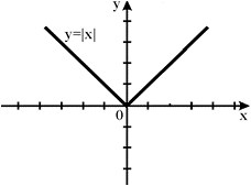
Function Graph y = |x| as follows:

Graphs of periodic (trigonometric) functions

Function at = f(x) is called periodical, if there exists such a non-zero number T, what f(x + T) = f(x), for anyone X out of function scope f(x). If the function f(x) is periodic with period T, then the function:

where: A, k, b are constant numbers, and k not equal to zero, also periodic with a period T 1 , which is determined by the formula:

Most examples of periodic functions are trigonometric functions. Here are the graphs of the main trigonometric functions. The following figure shows part of the graph of the function y= sin x(the whole graph continues indefinitely to the left and right), the graph of the function y= sin x called sinusoid:

Function Graph y= cos x called cosine wave. This graph is shown in the following figure. Since the graph of the sine, it continues indefinitely along the OX axis to the left and to the right:

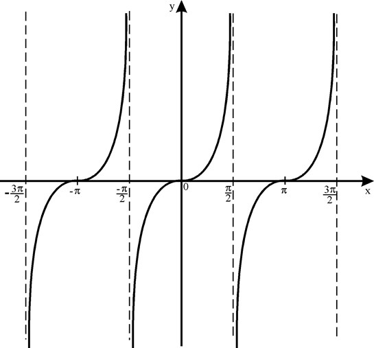
Function Graph y=tg x called tangentoid. This graph is shown in the following figure. Like the graphs of other periodic functions, this graph repeats indefinitely along the OX axis to the left and to the right.

And finally, the graph of the function y=ctg x called cotangentoid. This graph is shown in the following figure. Like the graphs of other periodic and trigonometric functions, this graph repeats indefinitely along the OX axis to the left and to the right.

Successful, diligent and responsible implementation of these three points will allow you to show an excellent result on the CT, the maximum of what you are capable of.

Found an error?

If you, as it seems to you, found an error in the training materials, then please write about it by mail. You can also write about the error on the social network (). In the letter, indicate the subject (physics or mathematics), the name or number of the topic or test, the number of the task, or the place in the text (page) where, in your opinion, there is an error. Also describe what the alleged error is. Your letter will not go unnoticed, the error will either be corrected, or you will be explained why it is not a mistake.

Elementary functions and their graphs

Straight proportionality. Linear function.

Inverse proportion. Hyperbola.

quadratic function. Square parabola.

Power function. Exponential function.

logarithmic function. trigonometric functions.

Inverse trigonometric functions.

Please draw a square parabola for the case a > 0, D > 0 .

Main characteristics and properties of a square parabola:

Function scope:  < x+ (i.e. x R ), and the area

values: … (Please answer this question yourself!);

The function as a whole is not monotonic, but to the right or left of the vertex

behaves like a monotone;

The function is unbounded, everywhere continuous, even for b = c = 0,

and non-periodic;

- at D< 0 не имеет нулей. (А что при D 0 ?) .

Functions y= Arcsin x(fig.23) and y= Arccos x(fig.24) many-valued, unlimited; their domain of definition and range of values, respectively: 1 x+1 and  < y+ . Since these functions are multivalued,